Transfer Learning in Deep Learning Using Tensorflow 2.0

Nov 16, 2020 • 12 Minute Read

Overview

TensorFlow is one of the top deep learning libraries today. A previously published guide, Transfer Learning with ResNet, explored the Pytorch framework. This guide will take on transfer learning (TL) using the TensorFlow library. The TensorFlow framework is smooth and uncomplicated for building models.

In this guide, you will learn how to use a pre-trained MobileNet model using TensorFlow Hub (TFHub), a library for the publication, discovery, and consumption of reusable parts of machine learning models.

You'll use a dataset from Kaggle to predict whether images depict aliens or predators. Click here to download the dataset.

Why MobileNet?

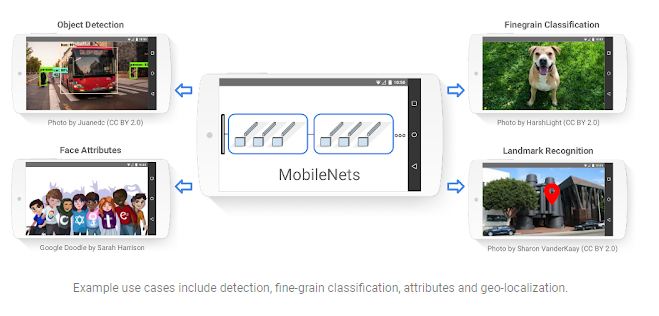
Computer vision networks have the responsibility to make a deeper network achieve higher accuracy. In short, the deeper the model, the harder it is to optimize. For compact applications, it becomes inconvenient to maintain the number of operations as the system has limited computation and power.

MobileNet was introduced to mitigate these problems. It has two versions, MobileNet-V1 and MobileNet-V2. This guide will stick to MobileNet-V2. Compared to other models, such as Inception, MobileNet outperforms with latency, size, and accuracy. To build lighter deep neural networks, it uses Depthwise Separable Convolution (DSC) layers.

MobileNet Architecture

The main aim of TL is to implement a model quickly. There will be no change in the MobileNet architecture whatsoever. The model will transfer the features it has learned from a different dataset that has performed the same task.

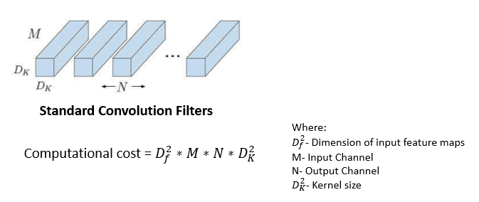
While applying the composite function in the standard convolution layer, the convolution kernel is applied to all the channels of the input image and slides the weighted sum to the next pixel. MobileNet uses this standard convolution filter on only the first layer.

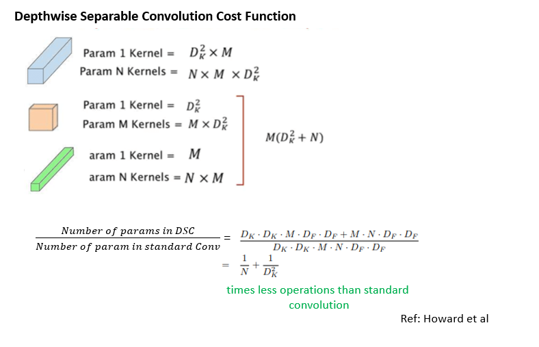
Depthwise Separable Convolution

The next layer is depthwise separable convolution, which is the combination of depthwise and pointwise convolution.

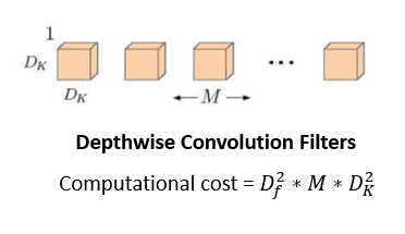
Depthwise Convolution

Unlike standard convolution, a depthwise convolution maps only one convolution on each input channel separately. The channel dimension of the output image (3 RGB) will be the same as that of an input image.

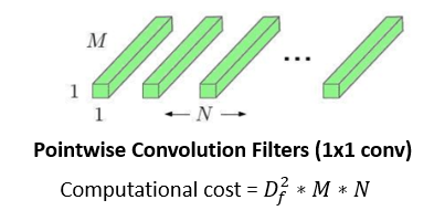
Source: Thermal Stresses—Advanced Theory and Applications

Pointwise Convolution

This is the last operation of the filtering stage. It's more or less similar to regular convolution but with a 1x1 filter. The idea behind pointwise convolution is to merge the features created by depthwise convolution, which creates new features.

Source: Thermal Stresses—Advanced Theory and Applications

The cost function of DSC is the sum of the cost of depthwise and pointwise convolution.

Other than this, MobileNet offers two more parameters to reduce the operations further:

Width Multiplier: This introduces the variable α ∈ (0, 1) to thin the number of channels. Instead of producing N channels, it will produce αxN channels. It will choose 1 if you need a smaller model.
Resolution Multiplier: This introduces the variable ρ ∈ (0, 1), it is used to reduce the size of the input image from 244, 192, 160px or 128px. 1 is the baseline for image size 224px.

You can train the model on a 224x224 image and then use it on 128x128 images as MobileNet uses Global Average Pooling and doesn't flatten layers.

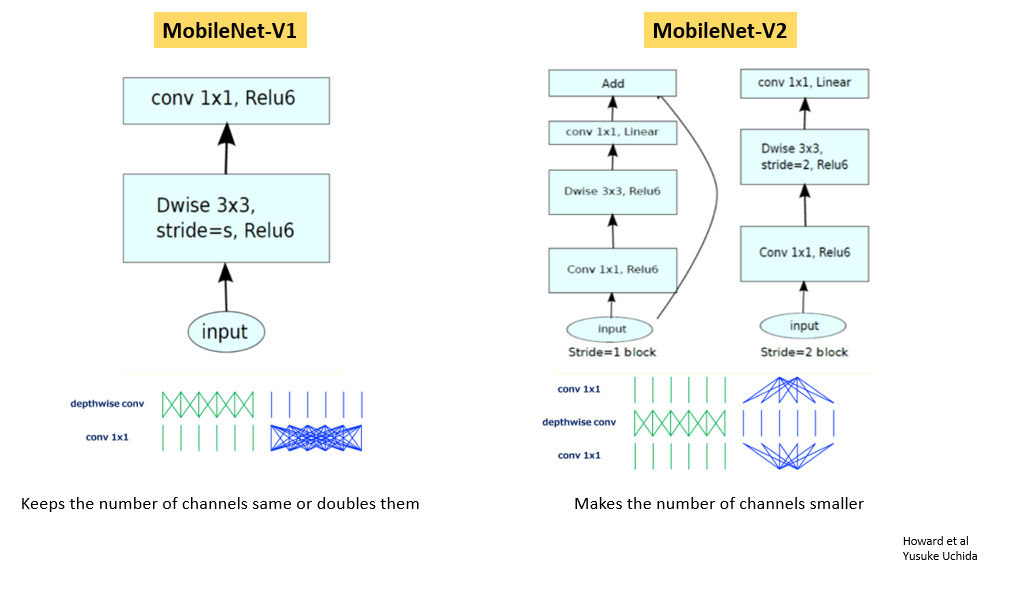
MobileNet-V2

The MobileNet-V2 pre-trained version is available here. Its weights were initially obtained by training on the ILSVRC-2012-CLS dataset for image classification (Imagenet).

The basic building blocks in MobileNet-V1 and V2:

The final MobileNet-V2architecture looks like this:

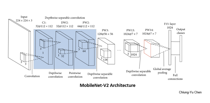
https://www.hindawi.com/journals/misy/2020/7602384/

Build a MobileNet Model

Now that you know the elements of MobileNet, you can build the model from scratch to make it more customize or use the pre-trained-model and save some time.

Let's see how the code works. Start with importing the essential libraries.

      import os 
import tensorflow as tf
import tensorflow_hub as hub
from tensorflow.keras import layers, Sequential
import tensorflow.keras.backend as K
from tensorflow.keras.preprocessing import image
from tensorflow.keras.preprocessing.image import ImageDataGenerator
from tensorflow.keras.callbacks import EarlyStopping
import pathlib
import matplotlib.pyplot as plt
import seaborn as sns
sns.set()
import numpy as np
    

      train_root = "../alien-vs-predator-images/train"
test_root = "../alien-vs-predator-images/validation"
    

      image_path = train_root + "/alien/103.jpg"
def image_load(image_path):
    loaded_image = image.load_img(image_path)
    image_rel = pathlib.Path(image_path).relative_to(train_root)
    print(image_rel)
    return loaded_image
    

Testing the above function:

      image_load(image_path)

The data seems ready. But to use it, you need load it into the model.

      train_generator = ImageDataGenerator(rescale=1/255) 
test_generator = ImageDataGenerator(rescale=1/255) 

train_image_data = train_generator.flow_from_directory(str(train_root),target_size=(224,224))
test_image_data = test_generator.flow_from_directory(str(test_root), target_size=(224,224))
    

TFHub also distributes models without the top classification layer. It uses feature_extractor for transfer learning.

      # Model-url
feature_extractor_url = "https://tfhub.dev/google/imagenet/mobilenet_v2_100_224/feature_vector/2"
    

      def feature_extractor(x):
  feature_extractor_module = hub.Module(feature_extractor_url)
  return feature_extractor_module(x)

IMAGE_SIZE = hub.get_expected_image_size(hub.Module(feature_extractor_url))
IMAGE_SIZE
    

      for image_batch, label_batch in train_image_data:
    print("Image-batch-shape:",image_batch.shape)
    print("Label-batch-shape:",label_batch.shape)
    break
    

      for test_image_batch, test_label_batch in test_image_data:
    print("Image-batch-shape:",test_image_batch.shape)
    print("Label-batch-shape:",test_label_batch.shape)
    break
    

      feature_extractor_layer = layers.Lambda(feature_extractor,input_shape=IMAGE_SIZE+[3])
    

Freeze the variables in the feature extractor so that training only modifies the new classifier layer.

      feature_extractor_layer.trainable = False

      model = Sequential([
    feature_extractor_layer,
    layers.Dense(train_image_data.num_classes, activation = "softmax")
    ])
model.summary()
    

Next, initialize the TFHub module.

      sess = K.get_session()
init = tf.global_variables_initializer()

sess.run(init)
    

Test a single image.

      result = model.predict(image_batch)
result.shape
    

      (32, 2)

The next step is to compile the model with an optimizer.

      model.compile(
    optimizer = tf.train.AdamOptimizer(),
    loss = "categorical_crossentropy",
    metrics = ['accuracy']
    )
    

Create a custom callback to visualize the training progress during every epoch.

      class CollectBatchStats(tf.keras.callbacks.Callback):
  def __init__(self):
    self.batch_losses = []
    self.batch_acc = []
    
  def on_batch_end(self, batch, logs=None):
    self.batch_losses.append(logs['loss'])
    self.batch_acc.append(logs['acc'])
    
# Early stopping to stop the training if loss start to increase. It also avoids overfitting.
es = EarlyStopping(patience=2,monitor="val_loss")
    

Then, use CallBacks to record accuracy and loss.

      batch_stats = CollectBatchStats()
# fitting the model
model.fit((item for item in train_image_data), epochs = 3,
         steps_per_epoch=21,
         callbacks = [batch_stats, es],validation_data=test_image_data)
    

Now, get the ordered list of labels.

      label_names = sorted(train_image_data.class_indices.items(), key=lambda pair:pair[1])
label_names = np.array([key.title() for key, value in label_names])
label_names
    

You're almost finished. Run predictions for the test batch.

      result_batch = model.predict(test_image_batch)

labels_batch = label_names[np.argmax(result_batch, axis=-1)]
labels_batch
    

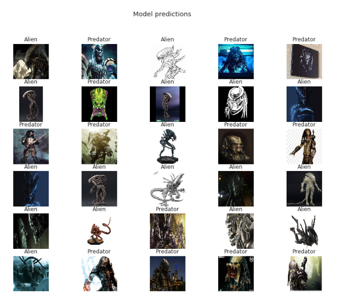
And finally, show the predicted results.

      plt.figure(figsize=(13,10))
for n in range(30):
  plt.subplot(6,5,n+1)
  plt.imshow(test_image_batch[n])
  plt.title(labels_batch[n])
  plt.axis('off')
  plt.suptitle("Model predictions")
    

You may save the model for later use.

Conclusion

Well done! The accuracy is ~94%. Your small but powerful NN model is ready. The trade-off between performance and speed is acceptable unless it is deployable on an embedded device and gives real-time offline detection.

To have good control of building the models, I recommend running the code on different datasets. Notice the accuracy and run time. This guide has given you a brief explanation of how to use pre-trained models in the TensorFlow library and MobileNet architecture. Read the links mentioned in the guide for a better understanding. You can create compact and insanely fast classifiers using MobileNets. They are widely used in NLP applications.

If you have any questions, feel free to reach out to me at CodeAlphabet.