Explore R Libraries: tidydice

Sep 14, 2020 • 7 Minute Read

Introduction

When you were in high school, you probably studied basic statistics using virtual experiments like flipping a coin, rolling dice, or selecting a certain number of cards. When you start your career in data analysis, you will frequently encounter various situations where you might need to recall those experiments to help you learn various statistical topics, such as probability distributions, moments, the law of large numbers, and so on. If you are an R user, you can benefit from the tidydice library, which presents automated results of rolling a die and flipping a coin.

In this guide, you will learn to perform these simulations and plot their binomial distribution.

Basics

Download and install the tidydice library with the following command:

      install.packages("tidydice")

If your internet proxy doesn't interfere in downloading the package and you have system permission to save the package in your drive, you should receive the following success message along with other information:

package ‘tidydice’ successfully unpacked and MD5 sums checked

Next, load the package in your current R environment using the given code:

      library(tidydice)

Note: You can also install and load the tidyverse package, which goes hand in hand with the tidydice package.

Simulating Experiments Related to Flipping of a Coin

The tidydice package provides the flip_coin function with which you can conduct experiments. The code below, from R’s documentation, demonstrates a few of the possible variations of the flip_coin function.

      flip_coin(data = NULL, times = 1, rounds = 1, success = c(2),
  agg = FALSE, sides = 2, prob = NULL, seed = NULL)
    

The results are not expressed as Heads and Tails, but rather 1 and 2. By default, the coin is unbiased, but you can change its behavior by using the prob parameter. The code below demonstrates a few of the possible variations of the flip_coin function.

      # 1. Flipping a coin two times
flip_coin(times = 2)

# # A tibble: 2 x 5
# experiment round    nr result success
# <int> <int> <int> <int> <lgl>  
#   1     1     1      1 FALSE  
#   1     1     2      2 TRUE  


# 2. Flipping a coin two times for three rounds
flip_coin(times = 2, rounds = 3)

# # A tibble: 6 x 5
# experiment round    nr result success
# <int> <int> <int> <int> <lgl>  
#  1     1     1      2 TRUE   
#  1     1     2      1 FALSE  
#  1     2     1      1 FALSE  
#  1     2     2      1 FALSE  
#  1     3     1      2 TRUE   
#  1     3     2      2 TRUE  


# 3. Flipping a coin three times by inducing bias 
#     of 90% to one of the side
s
flip_coin(times = 3, prob = c(0.1, 0.9))

# # A tibble: 3 x 5
# experiment round    nr result success
# <int> <int> <int> <int> <lgl>  
# 1     1     1      1 FALSE  
# 1     1     2      2 TRUE   
# 1     1     3      2 TRUE  


# 4. Flipping a coin 5 times and reproducing 
#     the same results with every run
flip_coin(times = 5, seed = 42)

# # A tibble: 5 x 5
# experiment round    nr result success
# <int> <int> <int> <int> <lgl>  
# 1     1     1      1 FALSE  
# 1     1     2      1 FALSE  
# 1     1     3      1 FALSE  
# 1     1     4      1 FALSE  
# 1     1     5      2 TRUE   


# 5. Combining experiments of flipping coins
flip_coin(times = 3, seed = 41, agg = T) %>%
  flip_coin(times = 2, seed = 42, agg = T)

# # A tibble: 2 x 4
# experiment round times success
# <int> <int> <int> <int>
# 1     1     3       1
# 2     1     2       0
    

Simulating Experiments Related to Rolling a Die

The tidydice package provides great flexibility in simulating experiments of rolling a die by giving you not only a textual representation of results, but also graphical ones. The code below, from R’s documentation, demonstrates a few of the possible variations of the roll_dice function.

      roll_dice(data = NULL, times = 1, rounds = 1, success = c(6),
  agg = FALSE, sides = 6, prob = NULL, seed = NULL)
    

The parameters of this function are similar to that of the flip_coin function. By default, the die is fair and you can bring bias to any of the sides using the prob parameter. Also by default, success is set to side 6, so you will receive TRUE when the dice results in the value 6. You can update this information anytime.

Here are two experiments based on this function:

      # 1. Rolling a die four times with 50% bias to its third side 
#    and 10% to the rest of the sides. Also, providing a seed value
#    for reproducible results

roll_dice(times = 4, prob = c(0.1, 0.1, 0.5, 0.1, 0.1, 0.1), seed = 100)

# # A tibble: 4 x 5
# experiment round    nr result success
# <int> <int> <int>  <int> <lgl>  
#   1     1     1      3   FALSE  
#   1     1     2      3   FALSE  
#   1     1     3      6   TRUE   
#   1     1     4      3   FALSE  

# 2. Rolling a die 10 times and finding how many times 
#    the second side is rolled by setting the parameter 'success' to 2

roll_dice(times = 10, agg = TRUE, success = c(2), seed = 100)

# # A tibble: 1 x 4
# experiment round times success
# <int> <int> <int>   <int>
#   1     1    10       2
    

So far, you have learned how to generate tabular results of rolling a die. You can also get these results as a plot to make simulations more pleasant to the eye:

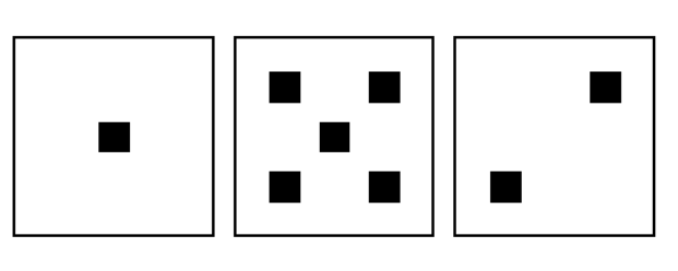
      # 1. Rolling a die 3 times with a seed value
roll_dice(times = 3, seed = 402) %>% 
  plot_dice()
    

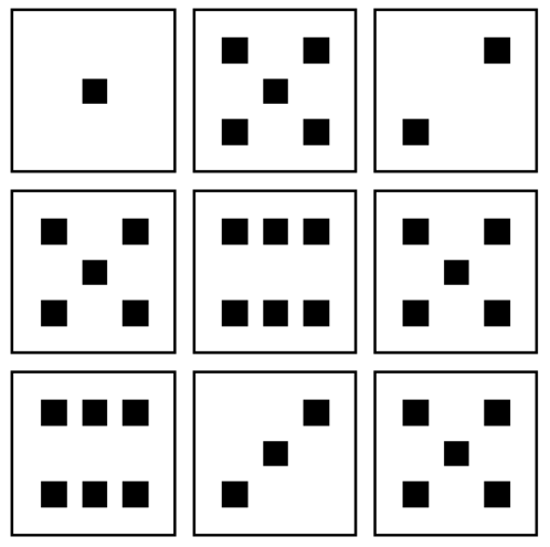
      # 2. Rolling a die 3 times in 3 rounds with a seed value
roll_dice(times = 3, rounds = 3, seed = 402) %>% 
  plot_dice()
    

Plotting a Binomial Distribution of your Experiment

You can plot the binomial distribution of your experiment using the command plot_binom.

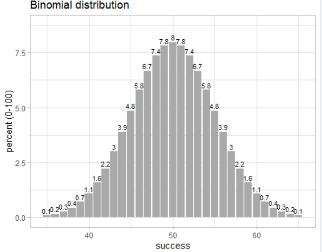
Binomial distribution of flipping a coin 100 times:

      binom_coin(times = 100) %>% plot_binom()

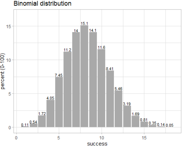
Binomial distribution of rolling a die 50 times:

      binom_dice(times = 50) %>% plot_binom()

Conclusion

In this guide, you learned how to create automated simulations related to flipping a coin and rolling a die (including creating a plot). You can use these simulations with other statistical packages in R or to revise your statistical concepts.