Explore R Libraries: Rpart

Jul 16, 2020 • 12 Minute Read

Introduction

Rpart is a powerful machine learning library in R that is used for building classification and regression trees. This library implements recursive partitioning and is very easy to use. In this guide, you will learn how to work with the rpart library in R.

Data

In this guide, you will use fictitious data of loan applicants containing 600 observations and eight variables, as described below:

Is_graduate: Whether the applicant is a graduate ("Yes") or not ("No")
Income: Annual Income of the applicant in USD
Loan_amount: Loan amount in USD for which the application was submitted
Credit_score: Whether the applicant's credit score is statisfactory ("Satisfactory") or not ("Not_Satisfactory")
approval_status: Whether the loan application was approved ("Yes") or not ("No")
Age: The applicant's age in years
Investment: Total investment in stocks and mutual funds in USD as declared by the applicant
Purpose: Purpose of applying for the loan

The first step is to load the required libraries and the data.

      library(plyr)
library(readr)
library(dplyr)
library(caret)
library(rpart)
library(rpart.plot)

dat <- read_csv("data.csv")

glimpse(dat)
    

Output:

      Observations: 600
Variables: 8
$ Is_graduate     <chr> "No", "Yes", "Yes", "Yes", "Yes", "Yes", "Yes", "Yes",...
$ Income          <int> 3000, 3000, 3000, 3000, 8990, 13330, 13670, 13670, 173...
$ Loan_amount     <dbl> 6000, 9000, 9000, 9000, 8091, 11997, 12303, 12303, 155...
$ Credit_score    <chr> "Satisfactory", "Satisfactory", "Satisfactory", "Not _...
$ approval_status <chr> "Yes", "Yes", "No", "No", "Yes", "No", "Yes", "Yes", "...
$ Age             <int> 27, 29, 27, 33, 29, 25, 29, 27, 33, 29, 25, 29, 27, 33...
$ Investment      <dbl> 9331, 9569, 2100, 2100, 6293, 9331, 9569, 9569, 12124,...
$ Purpose         <chr> "Education", "Travel", "Others", "Others", "Travel", "...
    

The output shows that the dataset has four numerical (labelled as int) and four character variables (labelled as chr). You will convert these into factor variables using the line of code below.

      names <- c(1,4,5,8)
dat[,names] <- lapply(dat[,names] , factor)
glimpse(dat)
    

Output:

      Observations: 600
Variables: 8
$ Is_graduate     <fct> No, Yes, Yes, Yes, Yes, Yes, Yes, Yes, Yes, Yes, No, Y...
$ Income          <int> 3000, 3000, 3000, 3000, 8990, 13330, 13670, 13670, 173...
$ Loan_amount     <dbl> 6000, 9000, 9000, 9000, 8091, 11997, 12303, 12303, 155...
$ Credit_score    <fct> Satisfactory, Satisfactory, Satisfactory, Not _satisfa...
$ approval_status <fct> Yes, Yes, No, No, Yes, No, Yes, Yes, Yes, No, No, No, ...
$ Age             <int> 27, 29, 27, 33, 29, 25, 29, 27, 33, 29, 25, 29, 27, 33...
$ Investment      <dbl> 9331, 9569, 2100, 2100, 6293, 9331, 9569, 9569, 12124,...
$ Purpose         <fct> Education, Travel, Others, Others, Travel, Travel, Tra...
    

Data Partition

The createDataPartition function is used to split the data into training and test data. This is called the holdout-validation method for evaluating model performance.

The first line of code below sets the random seed for reproducibility of results. The second line performs the data partition, while the third and fourth lines create the training and test set. Finally, the fifth line prints the dimension of the training and test data.

      set.seed(100)
trainRowNumbers <- createDataPartition(dat$approval_status, p=0.7, list=FALSE)
train <- dat[trainRowNumbers,]
test <- dat[-trainRowNumbers,]
dim(train); dim(test)
    

Output:

      1] 420   8

[1] 180   8

Feature Scaling

The numeric features need to be scaled because the units of the variables differ significantly and may influence the modeling process. The first line of code below creates a list that contains the names of numeric variables. The second line uses the preProcess function from the caret library to complete this task. The method employed is of centering and scaling the numeric features, and the preprocessing object is fit only to the training data.

The scaling is applied on both the train and test data partitions, which is done in the third and fourth lines of code below. The fifth line prints the summary of the preprocessed train set. The output shows that now all the numeric features have a mean value of zero.

      cols = c('Income', 'Loan_amount', 'Age', 'Investment')

pre_proc_val <- preProcess(train[,cols], method = c("center", "scale"))

train[,cols] = predict(pre_proc_val, train[,cols])
test[,cols] = predict(pre_proc_val, test[,cols])

summary(train)

Output:

      Is_graduate     Income         Loan_amount                 Credit_score
 No : 90     Min.   :-1.3309   Min.   :-1.6568   Not _satisfactory: 97  
 Yes:330     1st Qu.:-0.5840   1st Qu.:-0.3821   Satisfactory     :323  
             Median :-0.3190   Median :-0.1459                          
             Mean   : 0.0000   Mean   : 0.0000                          
             3rd Qu.: 0.2341   3rd Qu.: 0.2778                          
             Max.   : 5.2695   Max.   : 3.7541                          
 approval_status      Age               Investment            Purpose   
 No :133         Min.   :-1.7607181   Min.   :-1.09348   Education: 76  
 Yes:287         1st Qu.:-0.8807620   1st Qu.:-0.60103   Home     :100  
                 Median :-0.0008058   Median :-0.28779   Others   : 45  
                 Mean   : 0.0000000   Mean   : 0.00000   Personal :113  
                 3rd Qu.: 0.8114614   3rd Qu.: 0.02928   Travel   : 86  
                 Max.   : 1.8944843   Max.   : 4.54891
    

Model Building with rpart

The data is ready for modeling and the next step is to build the classification decision tree. Start by setting the seed in the first line of code. The second line use the rpart function to specify the parameters used to control the model training process.

The important arguments of the rpart function are given below.

formula: a formula that links the target variable to the independent features.
data: the data to be used for modeling. In this case, you are building the model on training data.
method: defines the algorithm. It can be one of anova, poisson, class or exp. In this case, the target variables is categorical, so you will use the method as class.
minsplit: the minimum number of observations that must exist in a node in order for a split to be attempted.
minbucket: the minimum number of observations in any terminal node. If only one of minbucket or minsplit is specified, the code either sets minsplit to minbucket*3 or minbucket to minsplit/3, as appropriate.

You will build the classification decision tree with the following argument:

      set.seed(100)

tree_model = rpart(approval_status ~ Is_graduate + Income + Loan_amount + Credit_score + Age + Investment + Purpose, data = train, method="class", minsplit = 10, minbucket=3)

You can examine the model with the command below.

      summary(tree_model)

Output:

      Call:
rpart(formula = approval_status ~ Is_graduate + Income + Loan_amount + 
    Credit_score + Age + Investment + Purpose, data = train, 
    method = "class", minsplit = 10, minbucket = 3)
  n= 420 

          CP nsplit rel error    xerror       xstd
1 0.60902256      0 1.0000000 1.0000000 0.07167876
2 0.06766917      1 0.3909774 0.3909774 0.05075155
3 0.01503759      3 0.2556391 0.2631579 0.04258808
4 0.01002506      6 0.2030075 0.2706767 0.04313607
5 0.01000000      9 0.1729323 0.2857143 0.04420254

Variable importance
     Purpose Credit_score          Age   Investment  Loan_amount       Income 
          46           31           17            2            2            1
    

An advantage of a decision tree is that you can actually visualize the model. This is done with the code below.

      prp(tree_model)

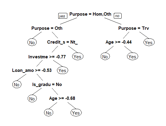
The above plot shows the important features used by the algorithm for classifying observations. The variables Purpose and Credit_score emerge as the most important variables for carrying out recursive partitioning.

Model Evaluation

You have built the algorithm on the training data and the next step is to evaluate its performance on the training and test dataset.

The code below predicts on training data, creates the confusion matrix, and finally computes the model accuracy.

      PredictCART_train = predict(tree_model, data = train, type = "class")

table(train$approval_status, PredictCART_train)

(131+266)/(131+266+23) #94.5%

Output:

      PredictCART_train
       No Yes
  No  131   2
  Yes  21 266
  
 (131+266)/(131+266+23) #94.5%
    

The accuracy on the training data is very good at 94.5%. The next step is to repeat the above step and check the model's accuracy on the test data.

      PredictCART = predict(tree_model, newdata = test, type = "class")

table(test$approval_status, PredictCART)

166/180 #92.2%

Output:

      PredictCART
       No Yes
  No   53   4
  Yes  10 113
  
  166/180  #92.2%
    

The output shows that the accuracy on the test data is 92%. Since the model performed well on both training and test data, it shows that the model is robust and its performance is good.

Conclusion

In this guide, you learned about the rpart library, which is one of the most powerful libraries in R to build non linear regression trees. You learned how to build and evaluate decision tree models, and also learned how to visualize the decision tree with the prp function.

To learn more about data science and machine learning with R, please refer to the following guides: