

Explore R Libraries: MICE
Jul 22, 2020 • 16 Minute Read
Introduction
Dealing with missing values is a common task for data scientists when building machine learning models. There are several methods of dealing with missing values, and if you want to use advanced techniques, the mice library in R is a great option.
MICE stands for Multivariate Imputation by Chained Equations, and it works by creating multiple imputations (replacement values) for multivariate missing data. The MICE algorithm can be used with different data types such as continuous, binary, unordered categorical, and ordered categorical data.
In this guide, you will learn how to work with the mice library in R.
Data
In this guide, you will use a fictitious data of loan applicants containing 600 observations and eight variables, as described below:
-
Is_graduate: Whether the applicant is a graduate ("Yes") or not ("No")
-
Income: Annual Income of the applicant (in USD)
-
Loan_amount: Loan amount (in USD) for which the application was submitted
-
Credit_score: Whether the applicant's credit score is satisfactory ("Satisfactory") or not ("Not_Satisfactory")
-
approval_status: Whether the loan application was approved ("Yes") or not ("No")
-
Age: The applicant's age in years
-
Investment: Total investment in stocks and mutual funds (in USD) as declared by the applicant
-
Purpose: Purpose of applying for the loan
The first step is to load the required libraries and the data.
      library(plyr)
library(readr)
library(dplyr)
library(caret)
library(mice)
library(VIM)

dat <- read_csv("C:/Notes_Old/A_Resources/data_qna/Content writing/R guides/caret package/data_mice.csv")

glimpse(dat)
Output:
      Observations: 600
Variables: 8
$ Is_graduate     <chr> "No", "Yes", "Yes", "Yes", "Yes", "Yes", "Yes", "Ye...
$ Income          <int> 3000, 3000, 3000, 3000, 8990, NA, NA, NA, NA, NA, N...
$ Loan_amount     <dbl> 6000, NA, NA, NA, 8091, NA, NA, NA, NA, NA, NA, NA,...
$ Credit_score    <chr> "Satisfactory", "Satisfactory", "Satisfactory", NA,...
$ approval_status <chr> "Yes", "Yes", "No", "No", "Yes", "No", "Yes", "Yes"...
$ Age             <int> 27, 29, 27, 33, 29, NA, 29, 27, 33, 29, NA, 29, 27,...
$ Investment      <dbl> 9331, 9569, 2100, 2100, 6293, 9331, 9569, 9569, 121...
$ Purpose         <chr> "Education", "Travel", "Others", "Others", "Travel"...
The output shows that the dataset has four numerical and four character variables. You will convert these into factor variables with the code below.
      names <- c(1,4,5,8)
dat[,names] <- lapply(dat[,names] , factor)
glimpse(dat)
Output:
      Observations: 600
Variables: 8
$ Is_graduate     <fct> No, Yes, Yes, Yes, Yes, Yes, Yes, Yes, Yes, Yes, No...
$ Income          <int> 3000, 3000, 3000, 3000, 8990, NA, NA, NA, NA, NA, N...
$ Loan_amount     <dbl> 6000, NA, NA, NA, 8091, NA, NA, NA, NA, NA, NA, NA,...
$ Credit_score    <fct> Satisfactory, Satisfactory, Satisfactory, NA, NA, S...
$ approval_status <fct> Yes, Yes, No, No, Yes, No, Yes, Yes, Yes, No, No, N...
$ Age             <int> 27, 29, 27, 33, 29, NA, 29, 27, 33, 29, NA, 29, 27,...
$ Investment      <dbl> 9331, 9569, 2100, 2100, 6293, 9331, 9569, 9569, 121...
$ Purpose         <fct> Education, Travel, Others, Others, Travel, Travel, ...
Missing Data Pattern Analysis
The summary() function provides a quick overview of the variables and missing values, if any.
summary(dat)
Output:
      Is_graduate     Income        Loan_amount                Credit_score
 No :130     Min.   :  3000   Min.   :  6000   Not _satisfactory:123
 Yes:470     1st Qu.: 39045   1st Qu.:115665   Satisfactory     :458
             Median : 50995   Median :135990   NA's             : 19
             Mean   : 65901   Mean   :149313
             3rd Qu.: 76170   3rd Qu.:170740
             Max.   :277770   Max.   :466660
             NA's   :20       NA's   :17
 approval_status      Age          Investment          Purpose
 No :190         Min.   :22.00   Min.   :  2100   Education: 94
 Yes:410         1st Qu.:35.00   1st Qu.: 16678   Home     :132
                 Median :50.00   Median : 26439   Others   : 64
                 Mean   :48.82   Mean   : 34442   Personal :174
                 3rd Qu.:61.00   3rd Qu.: 35000   Travel   :118
                 Max.   :76.00   Max.   :190422   NA's     : 18
                 NA's   :19
The output above shows that some of the variables have missing values, represented by NA's. To understand the pattern of missing values better, you can use the md.pattern() function.
md.pattern(dat)
Output:
      Is_graduate approval_status Investment Loan_amount Purpose
 559           1               1          1           1       1
 4             1               1          1           1       1
 4             1               1          1           1       1
 3             1               1          1           1       1
 10            1               1          1           1       0
 3             1               1          1           1       0
 2             1               1          1           0       1
 2             1               1          1           0       1
 1             1               1          1           0       1
 1             1               1          1           0       1
 6             1               1          1           0       1
 4             1               1          1           0       0
 1             1               1          1           0       0
               0               0          0          17      18

     Credit_score Age Income
 559            1   1      1  0
 4              1   0      1  1
 4              0   1      1  1
 3              0   1      0  2
 10             1   0      1  2
 3              1   0      0  3
 2              1   1      1  1
 2              1   1      0  2
 1              1   0      0  3
 1              0   1      1  2
 6              0   1      0  3
 4              0   1      0  4
 1              0   0      0  5
               19  19     20 93
The topmost row of the output indicates that there are 559 records with no missing values. There are 10 records that have missing values only in the Income variable, which overall has twenty missing values.
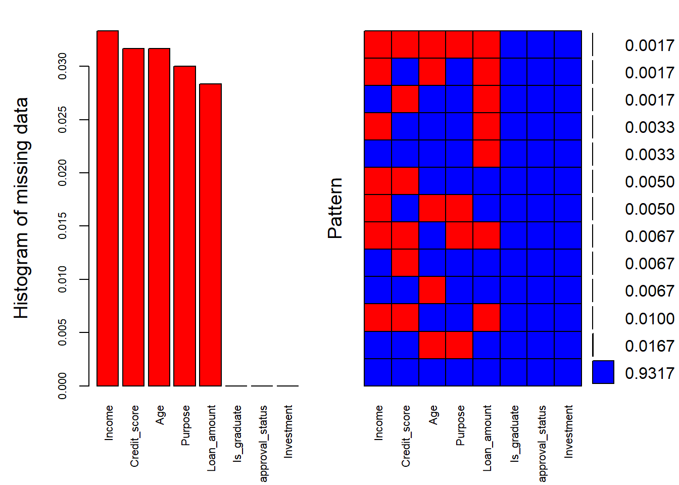
The missing value pattern can also be analyzed with the code below.
plot1 <- aggr(dat, col=c('blue','red'), numbers=TRUE, sortVars=TRUE, labels=names(dat), cex.axis=.7, gap=3, ylab=c("Histogram of missing data","Pattern"))
Output:
      Variables sorted by number of missings:
        Variable      Count
          Income 0.03333333
    Credit_score 0.03166667
             Age 0.03166667
         Purpose 0.03000000
     Loan_amount 0.02833333
     Is_graduate 0.00000000
 approval_status 0.00000000
      Investment 0.00000000
The output above prints the percentage of missing values in each of the variables. Overall, 93% of the data does not have missing values, which can be seen from the right-hand side plot below.
The number of missing values is not large, and you can remove these observations. But the objective is to use the mice library to treat missing values.
MICE Imputation
The mice() function is used to impute missing values. Some of the important arguments used in the code are explained below.
-
data: A data frame or a matrix containing the incomplete data. Missing values are coded as NA.
-
m: Number of multiple imputations. The default value is five.
-
method: Specifies the imputation method to be used for each column in data. In this case, you are using predictive mean matching (PMM) as an imputation method.
-
maxit: A scalar giving the number of iterations. The default value is five.
The above arguments are passed to the imputation function.
      imputed_data <- mice(dat,m=5,maxit=50,meth='pmm',seed=500)
summary(imputed_data)
Output:
      Class: mids
Number of multiple imputations:  5
Imputation methods:
    Is_graduate          Income     Loan_amount    Credit_score approval_status
             ""           "pmm"           "pmm"           "pmm"              ""
            Age      Investment         Purpose
          "pmm"              ""           "pmm"
PredictorMatrix:
                Is_graduate Income Loan_amount Credit_score approval_status Age
Is_graduate               0      1           1            1               1   1
Income                    1      0           1            1               1   1
Loan_amount               1      1           0            1               1   1
Credit_score              1      1           1            0               1   1
approval_status           1      1           1            1               0   1
Age                       1      1           1            1               1   0
                Investment Purpose
Is_graduate              1       1
Income                   1       1
Loan_amount              1       1
Credit_score             1       1
approval_status          1       1
Age                      1       1
If you want to look at a specific variable's imputed data—for instance, the variable Purpose—you can do that with the code below.
imputed_data$imp$Purpose
Output:
      1         2        3        4         5
 9      Travel Education   Travel Personal    Travel
 10  Education      Home     Home     Home      Home
 11       Home  Personal     Home     Home    Travel
 12       Home      Home   Travel     Home      Home
 13  Education Education   Travel   Travel      Home
 588    Travel    Others   Travel   Travel  Personal
 589    Travel    Travel Personal Personal  Personal
 590    Travel    Travel   Travel   Travel  Personal
 591    Travel  Personal   Travel   Travel    Others
 592    Travel  Personal   Travel   Travel Education
 593      Home Education Personal   Travel Education
 594      Home      Home     Home     Home      Home
 595  Personal Education   Travel   Travel Education
 596    Travel    Travel   Travel   Travel      Home
 597  Personal    Travel   Travel   Travel      Home
 598      Home Education   Travel   Travel Education
 599    Others  Personal Personal   Travel  Personal
 600    Others    Travel   Travel   Travel    Travel
The above output shows that for the 18 missing values in the Purpose variable, there are five sets of imputations available.
The next step is to complete the missing value imputation on the entire data with the code below. The missing values will be replaced with the values in the first of the five imputed datasets, indicated by the value of one in the second argument.
      completeddata1 <- complete(imputed_data,1)
summary(completeddata1)
Output:
      Is_graduate     Income        Loan_amount                Credit_score
 No :130     Min.   :  3000   Min.   :  6000   Not _satisfactory:129
 Yes:470     1st Qu.: 38498   1st Qu.:112973   Satisfactory     :471
             Median : 50835   Median :134385
             Mean   : 65819   Mean   :146552
             3rd Qu.: 76040   3rd Qu.:168715
             Max.   :277770   Max.   :466660
 approval_status      Age          Investment          Purpose
 No :190         Min.   :22.00   Min.   :  2100   Education: 96
 Yes:410         1st Qu.:35.00   1st Qu.: 16678   Home     :137
                 Median :50.00   Median : 26439   Others   : 66
                 Mean   :49.18   Mean   : 34442   Personal :176
                 3rd Qu.:61.25   3rd Qu.: 35000   Travel   :125
                 Max.   :76.00   Max.   :190422
The summary of the new data shows the absence of any missing values, indicating that the missing value imputation is complete. You can go ahead and use the new data for model building to check model performance on the imputed data.
Model Building with Imputed Data
The lines of code below create a data partition, build the random forest algorithm on the training data set, and evaluate the model on the test data set.
      # Create Data Partition
set.seed(100)
trainRowNumbers <- createDataPartition(completeddata1$approval_status, p=0.7, list=FALSE)
train <- completeddata1[trainRowNumbers,]
test <- completeddata1[-trainRowNumbers,]

# Build Random Forest Algorithm

control1 <- trainControl(sampling="rose",method="repeatedcv", number=5, repeats=5)
rf_model <- train(approval_status ~., data=train, method="rf", metric="Accuracy", trControl=control1)


# Model Evaluation
predictTest = predict(rf_model, newdata = test, type = "raw")
table(test$approval_status, predictTest)
Output:
      predictTest
       No Yes
  No   45  12
  Yes  11 112
The accuracy can be calculated from the above confusion matrix with the code below.
(112+45)/nrow(test)
Output:
1] 0.8722222
The output shows that the accuracy on the test data is 87%, which indicates that the model performance is good.
Conclusion
In this guide, you learned about the mice library, which is one of the advanced packages in R for missing value imputation. You learned how to identify and visualize the patterns of missing values in data, and to impute them with the mice librray. This will help you in data preprocessing and preparation for machine learning.
To learn more about data science and machine learning with R, please refer to the following guides:


Advance your tech skills today
Access courses on AI, cloud, data, security, and more—all led by industry experts.