

Explore Python Libraries: PyTorch
Jun 15, 2020 • 8 Minute Read
Introduction
Deep learning is one of the hottest topics in the field of machine learning and artificial intelligence. This guide will introduce you to PyTorch, a popular deep learning library from Facebook. PyTorch is positioned alongside TensorFlow from Google. Both PyTorch and TensorFlow have a common goal: training machine learning models using neural networks. But PyTorch offers a Pythonic interface to deep learning where TensorFlow is very low-level, requiring the user to know a lot about the internals of neural networks. Recently, the Keras project became part of TensorFlow, and some of the conveniences in PyTorch became available to TensorFlow users. However, Keras is higher level than even PyTorch. For many users, PyTorch may be the ideal compromise between flexibility and rapid development for training machine learning models.
A Network in PyTorch
A neural network in PyTorch is a class which inherits from torch.nn.Module. The layers of the network are declared in the class initializer.
      import torch.nn as nn
import torch.nn.functional as F

class Net(nn.Module):
    def __init__(self):
        super(Net, self).__init__()
        self.conv1 = nn.Conv2d(1, 32, 3, 1)
        self.conv2 = nn.Conv2d(32, 64, 3, 1)
        self.dropout1 = nn.Dropout2d(0.25)
        self.dropout2 = nn.Dropout2d(0.5)
        self.fc1 = nn.Linear(9216, 128)
        self.fc2 = nn.Linear(128, 10)
This is from the PyTorch examples and defines a simple network for the MNIST sample data set. Notice that the layers are only created and configured in the initializer. The connections between them are left for the forward method. This method takes the input (the image data), pushes it forward through the network, and returns a prediction.
      def forward(self, x):
    x = self.conv1(x)
    x = F.relu(x)
    # ...
    x = F.max_pool2d(x, 2)
    x = self.dropout1(x)
    # ...
    x = self.fc2(x)
    output = F.log_softmax(x, dim=1)
    return output
Redundant lines were omitted for brevity. But you can see the variable x always holds the current state of the prediction as it goes through the network. This is also how the activation functions are introduced.
Those familiar with Keras might be shocked at the amount of code needed to accomplish this. Many single line calls in Keras require multiple lines of code with PyTorch. But again, PyTorch gives you a level of control that Keras does not. On the other hand, PyTorch requires less code than the same task would if you were to use the lower level TensorFlow API.
Training a Model in PyTorch
Before training a PyTorch model, you must load a dataset from a DataLoader in the torch.utils.data module.
train_loader = torch.utils.data.DataLoader(torchvision.datasets.MNIST(...))
Often it is helpful to leverage a GPU when training a model with a neural network. A GPU must be enabled explicitly in PyTorch.
device = torch.device("cuda" if use_cuda else "cpu")
And then use the device when creating a new network.
model = Net().to(device)
The actual training requires an optimizer.
optimizer = torch.optim.Adadelta(...)
Then iterate over the DataLoader and train the model.
for _, (data, target) in enumerate(train_loader):
The data and target must be transferred to the GPU device.
data, target = data.to(device), target.to(device)
For each pass, the optimizer gradients are zeroed out.
optimizer.zero_grad()
A prediction is received from the model for the data. This is where the forward method is called.
output = model(data)
The functional module provides implementations of loss functions. The loss function will compare the predicted output to the expected target value.
loss = F.nll_loss(output, target)
Next comes the backpropagation step.
loss.backward()
And finally, the optimizer updates the model.
optimizer.step()
After multiple passes over the training data, the model can be tested using a similar method, but without computing the gradients. Once the model is accurate enough, saving it is simple.
torch.save(model.state_dict(), 'mnist.pt')
Obviously, this is much more code than is required for Keras. The equivalent code in Keras could be just one line. But there are other advantages to using PyTorch.
PyTorch Tensors
Data in PyTorch is stored in a Tensor.
x = torch.tensor([[2, 3], [5, 7]])
Conceptually, a tensor is a multidimensional list that knows a few new tricks. In the data science community, these are often created with numpy. An advantage that PyTorch has over TensorFlow is the ability to seamlessly move between tensor and numpy.array.
np_array_x = x.numpy()
And you can also easily create a tensor from a numpy.array.
      import numpy as np
y = np.random.randint(0, 10, size=(2, 3))
tensor_y = torch.from_numpy(y)
Dynamic Computational Graphs
In deep learning, the computational graph is similar to a flow chart. The nodes of the chart can represent operations, such as mathematical functions, or variables.
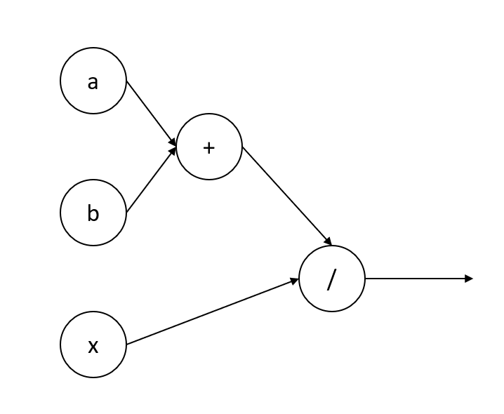
Here the computation graph would be the same as the function (a + b) / x. In PyTorch, the computational graph is created during training. This way the graph can be tuned to the training data. Static computational graphs assume that all data has the same size and structure. Traditionally TensorFlow has used static computational graphs. TensorFlow 2.0 has added some dynamic features, but older code will still use static graphs.
The computational graph is created by a technique called automatic differentiation implemented in the autograd module in PyTorch. During the forward pass of the network the computational graph will be created. This makes the backpropagation step a simple method call. Operations in the graph can be tracked by calling the method requires_grad_ on a Tensor and passing True to start tracking. When the backward method is called during training, the gradients are calculated for each operation that is being tracked. The tracking can be turned off for an entire graph with the no_grad method to speed up execution, for example, during testing of the model.
ONNX
ONNX is a standard for persisting machine learning models. PyTorch supports exporting models to the ONNX format. Many other deep learning libraries, including TensorFlow, can import ONNX models. This way, you can take advantage of the features for training models found in PyTorch, but use the models in projects leveraging other libraries. This is especially important for transfer learning.
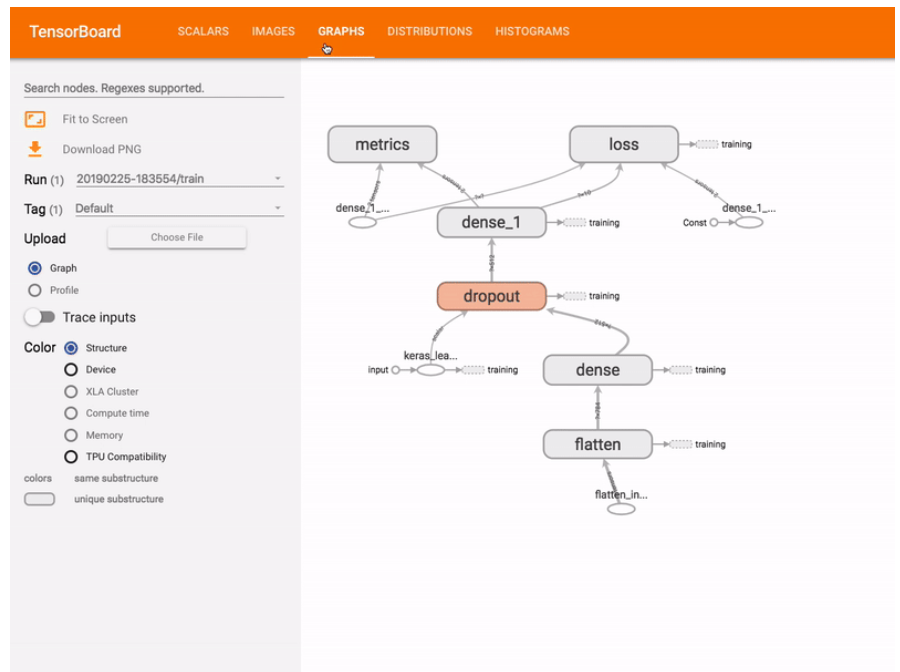
TensorBoard
Conclusion
PyTorch is a good fit for projects that don't need the complexity of TensorFlow, but need more control than Keras. This doesn't mean Keras should be avoided all the time. Keras is used by professionals in both research and industry. But Keras makes assumptions that don't apply to every situation. PyTorch lets you customize neural networks to meet the requirements of your project while still taking advantage of Python language features. Thanks for reading!


Advance your tech skills today
Access courses on AI, cloud, data, security, and more—all led by industry experts.